Time Series
Jun 2, 2025
LSTMs vs Transformers: What Works Best for Time-Series Forecasting? compares two leading deep learning models for sequence prediction. It explores the strengths of LSTMs—ideal for small datasets and short-term forecasting—and the power of Transformers, which excel at capturing complex, long-range patterns using self-attention. With practical examples and tool recommendations, the guide helps practitioners choose the right model based on data size, interpretability needs, and forecasting complexity.
Introduction
Time-series forecasting is one of the most valuable yet challenging tasks in machine learning. It powers real-world decisions in:
— Energy (predicting electricity demand)
— Retail (forecasting product sales)
— Automotive (scheduling car maintenance)
— Finance (modeling market risk and stock prices)
Time-series data is different from typical data. It changes over time and often includes unexpected problems like:
— Events must be understood in order — you can't just shuffle time
— Missing timestamps — sensors may fail or logs may skip steps
— Random spikes and dips — noisy outliers can confuse the model
— Peeking into the future by mistake — a common evaluation error
For years, the go-to models for this were RNNs and LSTMs. But now, Transformers are redefining what's possible.
What Makes Time-Series Forecasting Unique?
Let’s quickly look at what makes time-series challenging:
— Time matters — what happened before affects what happens next
— Patterns repeat — some signals are seasonal (daily, weekly, etc.)
— Irregular timing — some data points arrive late or go missing
— You can’t randomize — unlike typical data, you must keep the order
The model needs to both understand time and deal with messy, real-world signals.
How RNNs and LSTMs Work (and Why They’ve Been Trusted So Long)
Recurrent Neural Networks (RNNs) are built for sequences. They process one time step at a time and carry forward memory using a "hidden state."
However, RNNs often forget earlier inputs in long sequences — a problem called the vanishing gradient.
To fix this, Long Short-Term Memory (LSTM) networks add gates and a cell state to help manage what to remember, update, or discard.
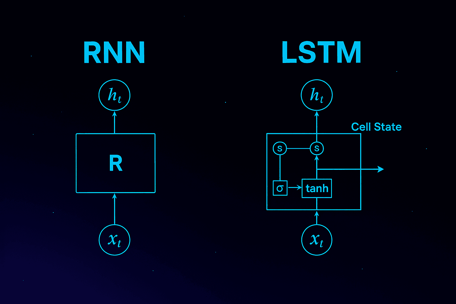
Imagine a looping arrow representing RNNs, where each output depends only on the immediate previous state.
Now picture LSTMs as a similar loop, but with added "gates" and a thick parallel line above: the cell state carrying long-term memory.
RNNs pass hidden states step by step. LSTMs add gates and a memory cell to retain long-term context.
Symbol | Meaning | Role |
xt | Input at time t | Example: today's sales |
ht | Hidden state | Short-term memory |
Ct | Cell state | Long-term memory |
σ | Sigmoid function | Controls what to pass or forget |
tanh | Hyperbolic tangent | Squashes values to -1 to 1 |
×, + | Multiply/Add | Used for gating and updates |
LSTM Strengths:
— Great for small to medium datasets
— Simple to deploy on edge or embedded devices
— Captures short-term patterns well
LSTM Limitations:
— Learns step-by-step — slow for long sequences
— Can’t handle very long-term dependencies well
— Harder to interpret compared to attention-based models
Enter Transformers: Sequence Modeling Without Recurrence
Transformers revolutionized sequence modeling with self-attention — a way for the model to analyze the entire sequence in parallel rather than step-by-step.
Instead of a loop like RNNs, imagine a full matrix of lines connecting every point in the sequence to every other point.
This is self-attention — and it’s what allows Transformers to model relationships across time instantly.

Self-Attention, Explained
Self-attention is the mechanism that allows Transformers to determine which parts of a sequence are important — for every time step, it calculates relevance scores for all others.
Picture a grid where each cell shows how much “attention” time step A pays to time step B.
Brighter cells = stronger relationships.
Key Concepts
Symbol | Meaning | Role |
Q | Query | What each step wants to understand |
K | Key | What each step offers |
V | Value | The actual content of the step |
α | Attention weight | Score of how important each input is |
+ | Residual addition | Adds back original input |
tanh | Activation | Optional non-linearity (rare in SA) |
Step-by-Step Breakdown
Project inputs into Q, K, and V vectors:
Q = XW^Q K = XW^K V = XW^V
Calculate attention scores (dot product of Q and K):
score(Qₐ, Kₑ) = Qₐ · Kₑ^T
Visualize a grid of scores — how similar is each query to each key?
Apply softmax to turn scores into probabilities:
αₐₑ = softmax(Qₐ · Kₑ^T)
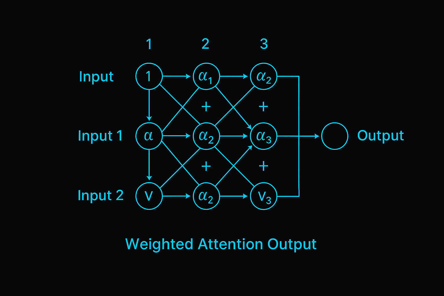
Use these weights to compute a new output as a weighted average of V:
Zₐ = ∑ αₐₑ Vₑ
This is where the model “pays attention” — weighting important values more.
Why This Works So Well
Compared to LSTMs, Transformers can:
— Access information from any point in time — instantly
— Learn long-range dependencies naturally
— Be trained in parallel, speeding up processing
Multi-Head Self-Attention
Transformers don’t just compute self-attention once. They do it multiple times in parallel, with each version (or "head") learning a different type of relationship.
MultiHead(Q, K, V) = Concat(head_1, ..., head_h)W^O
Imagine several attention maps running side-by-side. Some focus on short-term patterns, others on trends or seasonal cycles.

Multiple attention heads capture different temporal dynamics and are merged for the final output.
Real-World Example
Let’s say you want to forecast ride-hailing demand across 500 cities. Your input data includes:
— Time of day and day of week
— Local weather conditions
— Holidays or big events
— Previous week’s demand
A Transformer can weigh all of these signals — even those far apart in time — and model how they influence demand today and in the future. LSTMs would struggle with this breadth unless manually engineered to compensate.
LSTM vs Transformer: Head-to-Head
Feature | LSTM | Transformer |
Long-term memory | Limited | Excellent |
Training speed | Fast (step-by-step) | Slower per step, but parallelizable |
Memory usage | Low | High (especially for long sequences) |
Small dataset support | Strong | Needs more data |
Interpretability | Weak | Good (via attention weights) |
When to Use Which Model
Use LSTM if:
— You’re working with a small dataset
— You only need short-term predictions
— Your app must run on mobile or embedded systems
— You want fast setup and training
Use Transformer if:
— You have a large dataset
— Forecasting long into the future
— Your inputs include many variables
— You want interpretability and model depth
Tools That Support Both Keras (TensorFlow)
from tensorflow.keras.models import Sequential
from tensorflow.keras.layers import LSTM, Dense
model = Sequential([
LSTM(64, input_shape=(timesteps, features)),
Dense(1)
])
model.compile(optimizer='adam', loss='mse')
For Transformers: use keras_nlp, HuggingFace, or write custom attention blocks.
Other Libraries:
Darts: Forecasting library supporting LSTM, Transformer, Prophet, and N-BEATS
PyTorch Forecasting: Includes Temporal Fusion Transformer (TFT), embeddings, and backtesting tools
GluonTS (Amazon): Transformer + DeepAR for probabilistic forecasting
Kats (Meta): Supports forecasting, anomaly detection, signal decomposition
Final Takeaways
— LSTMs are lightweight and reliable for short-term, low-data problems
— Transformers are powerful for modeling complex, long-range dependencies
— The future likely lies in hybrid models that blend attention and memory (e.g., TransformerXL, RETAIN)
Common Pitfalls in Time-Series Forecasting
— Leaking future data into the training set
— Ignoring seasonality or trend components
— Using models that assume regular time intervals
— Randomly shuffling time-series data
— Underfitting due to missing features